
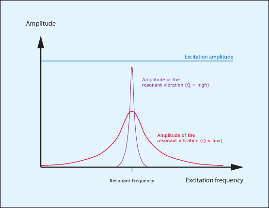
Most physical objects vibrate at frequencies determined by their size, shape, materials and construction, and the specific frequencies for each object are known as its resonant frequencies. Nonetheless, simply adding energy to an object doesn’t guarantee that you’ll obtain an output. Imagine an object having a single resonance of 400Hz placed in front of a speaker emitting a continuous note at, say, 217Hz. If you can picture it, the object tries to vibrate when the sound first hits it, but each subsequent pressure wave is received at the ‘wrong’ time so no sympathetic vibration is established. Conversely, image the situation in which the speaker emits a note at 400Hz. The object is now in a soundfield that it is pushing and pulling it at exactly the frequency at which it wants to vibrate, so it does so, with enthusiasm.
This suggests a simple rule: if an object is excited at one of its resonant frequencies, it will vibrate in sympathy; if it is excited at a different frequency, it won’t. But what might the situation be if this object found itself in a soundfield that had a frequency of 399.9Hz or 400.1Hz? Would it refuse to vibrate, or would the excitation be close enough to 400Hz to establish a certain amount of sympathetic vibration? Depending on the nature of the object, it would indeed vibrate to some degree, and there is a mathematical term (called ‘Q’) that describes the relationship between the excitation (the input signal), the resonant frequency of the object, and the amplitude of the sympathetic vibration (the output). If the Q is low, the range of excitation that can elicit a response is wide; it the Q is high, the range is narrow. (Figure 1.)
Resonant filters
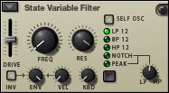
Interestingly, it’s not only physical objects that resonate; analogue circuits and digital algorithms can do so too, again creating a bump in their responses at their resonant frequencies. Indeed, there is a special type of filter called a Peaking Filter that does nothing but add a resonant peak to the signal spectrum, and you can find one of these in Thor’s State Variable Filter. However, this is a rare beastie, and you’re much more likely to encounter resonance in low-pass and high-pass filters, in which the resonant frequency is the same as the cut-off frequency, (There are good reasons why this should be so, but we won’t discuss them here because, as someone once said to me, “It’s obvious; it’s the solution to a second order differential equation.” Umm… right!)
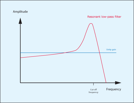
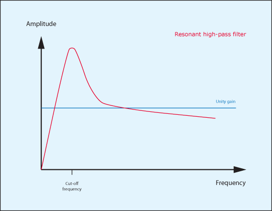
We can represent the response of a typical, resonant low-pass filter as shown in figure 2 and of a resonant high-pass filter as shown in figure 3. As you can see, the filters still attenuate the frequencies significantly above (LPF) or below (HPF) their cut-off frequencies, but in both cases a band around the cut-off frequency is boosted.
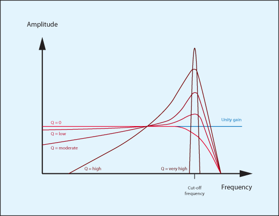
You might think that you could describe this response using two parameters – the cut-off frequency and the gain of the resonant peak – but there’s another attribute to consider – the ‘Q’ which, as before, describes the width of the peak. In fact, the width and the gain of a the resonance in a synthesiser’s filter are so closely related that, all other things being equal, a low Q means that the peak will be broad and low, whereas a high Q means that the peak will be narrow and high (figure 4) so only two controls are needed to control them: the cut-off frequency and the Q – or the “amount of resonance”.
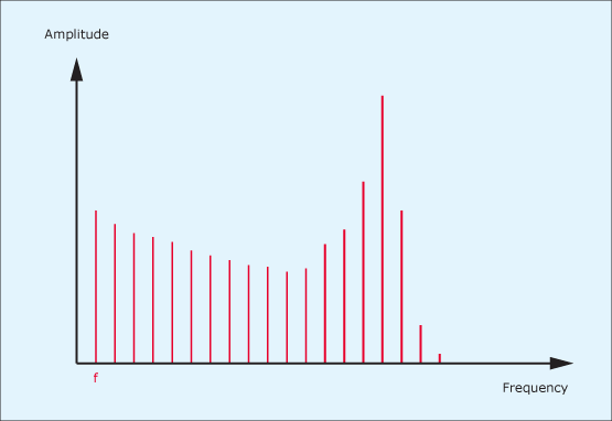
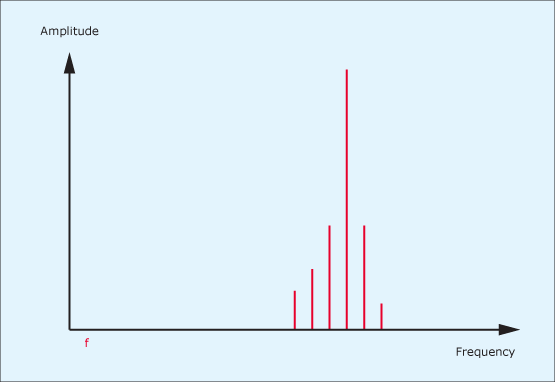
To illustrate the action of a resonant low-pass filter upon the spectrum of an harmonic audio signal, let’s consider one that I introduced in the previous tutorial, and which is shown again in figure 5. Passing this signal through a low-pass filter with a moderately high Q might result in the spectrum shown in figure 6. If the Q is increased further, you might obtain the spectrum shown in figure 7, which represents an enormous change in the nature of the sound. Clearly, the resonant filter is a much more powerful sound-shaping tool than the non-resonant low-pass and high-pass filters described in the previous two tutorials.

Using resonance to create sounds in Thor
In the first of these filter tutorials, I demonstrated how you could open and close one of Thor’s low-pass filters with a simple AD contour (figure 8) to make a single note change from a dull tone at the beginning of a note, to a much brighter one as the note progressed, and then back to the original tone at the end:

(Click to enlarge)
Now, without making any other changes to the patch, I’ll add filter resonance so that any of the note’s harmonics lying close to the cut-off frequency will be accentuated as the filter sweeps opens and then closes. (Figure 9.) Sound #2 was recorded with a resonance of 113:
While sound #3 had a resonance of 121:
Armed with resonance, you’re now in a position to adjust the envelope and filter parameters to create all manner of filter sweeps, blips and other popular ‘synth’ sounds. For example, the simple bass line in sound #4 was created by taking sound #3 and speeding up the Filter Env sweep by setting the Attack to zero and the Decay to around a second:
Fortunately, patches that use filter sweeps can be far more interesting than this. Sound #5 uses three sawtooth oscillators with one tuned an octave above the other two, all of which are detuned from one another to add ‘thickness’ to the sound. Then, as in the previous example, the Filter Env causes the filter’s cut-off frequency to reinitialise at its maximum value each time that you press a key, and to sweep downward during the course of the note to create its instantly recognisable character. (See figure 10.)

(Click to enlarge)
Interesting though this sound is, the Minimoog-style architecture of the patch (I’m sure that you guessed) would soon prove to be rather limited for creating some of the more complex sounds that rely on filter resonance. But in 1973 Korg introduced a series of affordable little synthesisers that offered not one but two resonant filters – a HPF followed by a LPF. In truth, the factory sounds for these synths (i.e. the printed patch charts that came with their manuals) made very little use of their resonant high-pass filters, but if they had one signature sound, it was the “analogue voice” that their dual-filter architecture made possible.
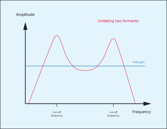
The human voice is defined in part by the presence of resonances known as formants. The positions of these and the way that they change during speech and singing are unique to each individual, which is why you can recognise people’s voices. Unfortunately, the smallest number of synthesised formants that can contribute to recognisable speech is three, but two can still recreate a semblance of a vocal sound. So, long before the appearance of digital synths with choir samples, we old-timers used dual HP- and LP- filters to create all manner of “synthvox” voices based upon the combined filters’ response shown in figure 11.
To create a synthvox patch, start by placing a single analogue oscillator in Thor’s Osc 1 slot, select the pulse wave and set its width to somewhere around 14. Next, create a gentle ASR amplitude contour using the Amp Env. Now place an HP12 filter in the Filter 1 slot and a LP12 filter in the Filter 2 slot, and set up the routing appropriately. With the filters wide open you obtain exactly what you would expect: the raw buzz of an untreated, narrow pulse wave :
Next, add some vibrato by using the modulation matrix to direct the output from LFO1 to the oscillator pitch. Ah… a wobbly buzz that sounds like a cheap combo organ:
Now filter the sound. Set the cut-off frequency of the high-pass filter to around 600Hz, and that of the low-pass filter to around 900Hz. Ah… a dull, wobbly buzz!
Now let’s do the clever bit and increase the resonance of both filters. I’ve chosen values that are high, but not at the very top of the range because this would make the sound ‘ring’. With the HPF resonance at 115 and the LPF resonance at 117 you’ll obtain sound #9 , which is very similar to the analogue ‘voices’ of the early 1970s. (See figure 12.)
Finally, add a bit (well, a lot) of an external ensemble effect and some reverb to obtain the ensemble in sound #10:
Now you need only play the right notes to invoke the Electric Monks in sound #11:

(Click to enlarge)
There are dozens of other classic sounds to be discovered when you start experimenting with multiple resonant filters, including emulations of musical instruments that cannot be synthesised by simple attenuation of high or low frequencies. At the other end of the spectrum (no pun intended) the quality of the bass sounds created by the Minimoog is a consequence of its unusual resonant response, and understanding this makes it possible to create much better emulations of this classic synth. In short, the amount of resonance is dependent upon the cut-off frequency, and there’s no emphasis when its filter cut-off frequency is below 150Hz or thereabouts. Happily, Thor allows you to imitate this by connecting the Note (Full Range) to the Filter Res in the modulation matrix… but I’ll leave you to try this for yourself.
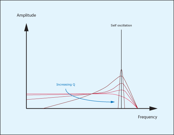
Self oscillation
Before leaving this discussion of resonance, let’s return for a moment to the idea of a resonant object being excited by something vibrating at its resonant frequency. In fact, let’s excite it with its own output. This isn’t as crazy as it might seem. When a guitarist plucks a string on an electric guitar with no amplification, the excitation set the string vibrating and you hear the acoustic response of the instrument. Now imagine turning the amp on and the volume up far enough that some of the note’s energy is injected back into the strings and the body of the guitar. If the amount of amplification is sufficient, a loop will be created; the string (with a bit of help from electricity) excites the air, which excites the string, which excites the air… round and round it goes, and the note can be sustained indefinitely. Depending upon a number of factors (but primarily the distance of the string from the speaker) a note can be sustained at any of the string’s resonant frequencies – it doesn’t need to be the note initially played – and no other frequencies are heard, so the Q is (in effect) infinite and the system is “self-oscillating”.
The same can be true of an analogue synthesiser’s filters. If the Q is great enough, the resonant peak will become so narrow and its gain will be so great that the slightest nudge will start it oscillating at its resonant frequency. (Figure 13.) In a virtual analogue synth, a bit of trickery is required to initiate the oscillation, but that’s no problem. Having done so, you can use the filter as an extra oscillator – for example, excellent three-drawbar organ sounds can be obtained from the single-oscillator Roland Juno series synths by using the sub-oscillator and oscillator as the 16′ and 8′ drawbars in the patch, and the self-oscillating filter as the 52/3′ drawbar. Played through a decent Leslie emulator, the results can be remarkable. Other sounds can be obtained by taking a patch with little or no resonance, and then by increasing this in and out of self-oscillation – either manually or under the control of an LFO or contour generator – to create special effects. Few analogue synthesisers offer voltage control over Q, but Thor allows you to control it using any modulation source (or sources) you choose. Sound #12 illustrates the simplest example of this, illustrating what happens to sound #1 when the Q of the filter rather than its cut-off frequency is controlled by the Filter Env. The instability as the filter reaches the point of self-oscillation (and again as it leaves it) is a particular interesting effect that can be also used creatively. Sorry… did somebody out there whisper “feedback guitar patch”? If not, somebody should have done!
So there you have it… resonance, or ‘Q’ or ‘quality’ or ’emphasis’ or ‘peak’ (depending upon the synthesiser manufacturer’s choice) can be much more than just the means for making analogue filters go “splat”, and I hope that these examples have given you an idea of the difference that it can make to your sounds. Whether you use it subtly or in a more heavy-handed, obvious way, learn to use it well, because it’s one of the most important tools in any analogue (or virtual analogue) synthesiser’s armoury.
Text by Gordon Reid


