
Frequency Modulation (FM) has become the bogeyman of synthesis. Whereas, in the 1960s, people quickly grasped the concepts of these new-fangled oscillators, filters and contour thingies, the second generation of players shied away from the concepts of FM, to the extent that most FM synths were used for little more than their presets and the professionally programmed sounds that you could buy for them. Even today, if you look closely at Thor’s refills, you’ll find very few patches based upon its FM Pair Oscillator. This is a great shame, because FM is a very elegant system capable of remarkable feats of sound generation. So, this time, I’m going to introduce you to the principles of FM, and show you how to create what may well be your first FM sound.
Let’s start by considering what happens when you change the frequency of a pure tone (which, in synthesiser parlance, is called a sine wave). If you increase it steadily, you hear the pitch glide upward until it exceeds the bandwidth of your system, or the limit of your hearing, and becomes inaudible. If you lower it steadily, the pitch decreases until the sound drops below the limit of your hearing. But if you vary it up and down slowly (using another sine wave as a modulator) you hear a very common musical effect: vibrato.
Now let’s increase the speed of the up/down modulation. At first, you hear a faster vibrato, but as the frequency of the modulator moves into the audio range, the vibrato effect disappears and a new tone replaces the original, the nature of which is determined by the relationship between the frequencies of the original sine wave (the “carrier”) and the modulating sine wave (the “modulator”), and the amplitude of the modulator. To prove this would mean delving into some rather nasty equations, but don’t panic… I’m not going to do this. Instead, I’m going to present you with the results that you would obtain if you had a degree in mathematics.
If you refer back to the second tutorial in this series, you’ll find that, if you modulate the amplitude of one oscillator (the carrier) of frequency ωc (the character ω means “the frequency” so ωc means “the frequency of the carrier”) using another oscillator (the modulator) of frequency ωm, the result is two new signals (called side-bands) with frequencies ωc + ωm (the sum) and ωc – ωm (the difference). So, if you increase ωm while ωc remains constant, the frequency of the sum increases, while the frequency of the difference decreases. We can express this in a very neat way in the following form…

… which means that “the frequencies of the side-bands are equal to the frequency of the carrier plus or minus the frequency of the modulator”.
Now let’s turn our attention to frequency – rather than amplitude – modulation. If you work through the maths, you’ll find that this also creates side-bands, but instead of generating just two of them, you obtain a series expressed as…

… where the symbol “n” is an integer number: 0, 1, 2, 3, 4… and so on.
To put this into English, each side-band lies at a frequency equal to the carrier frequency plus or minus an integer multiple of the modulator frequency. Since the value of “n” can be 0, 1, 2… or hundreds, or thousands, or millions … then, in theory, FM produces an infinite series of side-bands. This, as you might imagine, poses certain problems, as does the issue of “negative frequencies” when n.ωm is greater than ωc, but I’m going to ignore both of these issues until the next tutorial.
OK… we now know the frequencies at which the side-bands are generated, but what about their amplitudes? What is the spectral content of an FM-generated signal? Intuitively, it would seem sensible to suppose that, as you increase the depth of the modulation, the output signal would become more complex, and this indeed proves to be the case. Nevertheless, the relationship between the modulation depth and the output spectrum is not quite as simple as one might hope. It’s described by a thing called the modulation index, denoted by the character “β”, which is the ratio of the maximum change in the carrier frequency divided by the modulation frequency. As β changes, side-bands can be introduced, diminish, disappear altogether, or even reappear with inverted phase. But the overall picture is as described; the greater the amplitude of the modulation, the more complex the output signal becomes.

To illustrate this, figure 1 shows a case where β is low: in the region of 0.1 or less. The only significant side-bands are those closest to the Carrier frequency, and the result is similar to what you might obtain using Amplitude Modulation. But if β is significantly higher – say, in the region of 5 – we obtain a much broader series of side-bands, and a much more complex spectrum results. (Figure 2.)


The nature of the Modulation Index has an interesting consequence: if you want the tone of an FM-generated sound to be consistent as you play up and down the keyboard, you need all three of the modulator, the carrier, and the amplitude of the modulator to track by 100%. If you make the modulator amplitude track by more or less than this, the resulting sound will differ in tone from note to note.
We can now state the simple rules of FM synthesis as follows:
Rule #1:
The frequency of the modulator determines the spacing of the side bands in an FM-generated signal.
Rule #2:
The number of audible side-bands is determined by the modulation index, which can be described in general terms as the amplitude of the modulator divided by the frequency of the modulator.
Programming an FM sound
Inevitably, there are complications to this picture, but if you keep these rules in mind, you can programme useful FM sounds. Thor allows you to do so using a dedicated oscillator called an FM Pair Osc. This has two “operators” – a modulator (called Mod) which is permanently connected to the frequency modulation input of a carrier (happily, called Carrier). This is the simplest possible version of FM, and the way in which the operators are connected (called an Algorithm) is represented by figure 3.

Let’s start with a basic configuration of Thor, with a single FM Pair Osc inserted into the Osc3 slot. [It’s usual practice to place the audio output operator(s) at the bottom of the algorithm.] Set the Carrier and Mod values to “1”, set the FM amount to zero and create a simple organ-shaped Amp Env with maximum Sustain and a short Attack and Release to eliminate the clicks that would otherwise occur. (Figure 4.) If you now play a note, you’ll hear nothing but a sine wave… the aforementioned ‘pure tone’ that contains nothing but the fundamental of the note:

(Click to enlarge)
Now let’s introduce some frequency modulation. The FM knob in the FM Pair Osc determines the amount by which the Mod affects the Carrier, so if you turn this clockwise you’ll hear the tone change. Sound #2 was generated with the FM knob set to 12 o’clock, with everything else unchanged:
Figure 5 shows the waveform of this sound, and you can see clearly how the sine wave generated by the carrier is being pitch-shifted (i.e. stretched and compressed) by the modulator.

(Click to enlarge)
As you can hear, sound #2 is brighter than sound #1, so this tells us how we can programme FM sounds with a dynamic spectral content. Figure 6 shows a patch in which the Osc3 FM amount is being swept by the Mod Env generator. The contour has no Attack, but a moderate Decay that sweeps the amount of modulation from its maximum down to zero. Sound #3 demonstrates the effect that this creates:

(Click to enlarge)
This sounds to me like a very bad approximation to the tonal changes that occur during the course of a note played on an electro-mechanical piano. This shouldn’t surprise us; FM synthesis is famous for its so-called “DX piano” patches. The most popular of these used six operators but, remarkably, I’m now going to emulate these sounds using nothing more than a single FM Pair Osc!
The next stage is to adjust the Mod Env and the Amp Env in figure 6 to shape the changes in tone and volume in ways that are appropriate for an electric piano sound. I found that a Mod Env Decay of around a second is about right, with an Amp Env Decay of around four seconds. Why is the Mod Env contour shorter than the Amp Env’s? Well… think about the sound of a real piano or electric piano. When the hammer hits the string (or tine or reed) the sound contains a lot of high-frequency components, so it is initially bright, but the tone decays quickly to something more mellow, long before the note ends. The Mod Env is controlling the brightness, and the Amp Env is controlling the duration of the note, so all should now make sense.
Unfortunately, the sound that this produces is even more unrealistic than before. Sound #4 demonstrates that, even when played in a piano-like fashion, the result is horrendous:
Nonetheless, we’re on the right track. The problem is that (a) the amount of frequency modulation is too great, and (b) the patch contains no parameters that affect the tone as you play across the keyboard or as you change the dynamics of how you play.
Sorting out the first problem is easy. Reduce the FM modulation amount in the modulation matrix from 100 to around 40. Sound #5 shows that this is a dramatic improvement, and you may even be happy to use this patch as it is:
However, we’re currently in the territory of early 1970s non-sensitive electric pianos such as the Crumar Roadrunner and RMI Electrapiano, so I now need to look at how we can introduce timbral changes and dynamics.
The first thing to do is to add a modicum of velocity sensitivity to the tone by directing the Key Vel to the OSC3 FM Amt. This means that when you play a note harder (or, to be precise, with greater velocity) the tone is brighter than when you play it more softly:
Next, we can imitate a very important attribute of plucked and hammered instruments… that notes become shorter as they become higher pitched. We do this by adding another line in the modulation matrix to shorten the decays of the Mod Env and Amp Env as you play up the keyboard. Sound #7 , which was generated by the patch in figure 7, is now starting to show promise:

(Click to enlarge)
One of the things that makes this patch a tad unrealistic is that the notes at the top of the scale are too bright. Electric pianos have limited bandwidth and, because they dissipate their high frequency energy extremely quickly, the tines (or reeds) at the top end tend to be duller than you might otherwise expect. We can emulate this by adding another line in the modulation matrix that reduces the OSC3 FM Amount as you play up the keyboard.
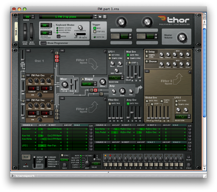
Next, I want to make the sound respond to the sustain pedal in a realistic way, so I have added yet another line that increases the length of the Amp Env Decay and Release when I press the pedal. This then leads to note stealing so we need to increase the polyphony to its maximum of 32 notes. We now obtain figure 8 and sound #8:

(Click to enlarge)
We’re nearly there, but the loudness of the sound is still insensitive to velocity, and we’re missing a very important effect that is crucial to the best e-piano sounds: panning tremolo. We can sort both of these out in the Amp section. First, we turn the Amp Vel knob fully clockwise so that MIDI Velocity affects the loudness of each note. Finally, we add yet another line to the modulation matrix that directs LFO1 to the pan of the amplifier. I find that an LFO rate of around 4Hz and a depth of a little less than maximum is rather pleasing. The resulting patch is shown in figure 9, and you can hear it in sound #9:

(Click to enlarge)
This is another remarkable result, and it demonstrates what can be done with just two operators. However, I’m now going to add a second FM Pair Osc to reinforce the fundamental of the sound. I’m not going to apply any FM modulation in this pair; the waveform it produces will simply be a sine wave at the fundamental frequency, somewhat quieter than the output from Osc3, but tuned upward by a few cents to create a slight thickening of the overall sound. The final patch, now with three operators, is shown in figure 10, and you can hear it in sound #10:
(Click to enlarge)
Before finishing, let’s look at the algorithm used in figure 10, which I have drawn as figure 11. As you can see, this is beginning to look very much like the graphics that you see on the control panels of Yamaha’s DX-series synths, and it leads us into a whole new area of FM synthesis; the use of multiple operators within a patch. But that will have to wait until next time. Until then…

Text & Music by Gordon Reid


